A study of temperature effects in the Bunter Closure 36, a potential large-scale CO₂ storage site in UK

The effect of temperature variation is discussed with reference to the Bunter Closure 36, a prospect considered for CO₂ storage in the UK. Although temperature is often considered as a secondary effect, it should not be neglected in an accurate CO₂ injection design.

Introduction

When selecting a storage site in deep saline aquifers, economic feasibility requires pressure and temperature conditions such that the CO₂ can be stored at a liquid-like density, to minimise the volume stored, and so maximise capacity, [1]. In many of the prospects studied around the world, the CO₂ is close to its critical point [31° C, 73.8 Bar], where small variations in temperature cause significant changes in density and viscosity. The viscosity impacts the mobility of the CO₂, while the density alters the volume occupied, with consequences on the footprint and the over-pressure during injection.

In general, CO₂ does not enter the aquifer at the initial aquifer temperature. However, the thermal capacity of the aquifer is such that the CO₂ being injected is quickly warmed-up or cooled-down to the ambient temperature. The thermal front generally lags behind the CO₂-brine interface, although its penetration depends on the type of injection. For multi-year prolonged injection, the injection temperature will travel further from the wells, while for intermittent injection the effect is more local. Either way, is worth observing that the CO₂ at storage conditions has a heat capacity close to that of a liquid, so the effect is greater than that of a gas such as methane. Away from the injection front, the natural geothermal temperature gradient of the aquifer is another cause of temperature variation that impacts the CO₂ properties.

The importance of thermal effects will vary from site to site, depending on the depth, vertical extension, difference between injection and aquifer temperature, and the way the site is operated.

The Bunter Closure 36 prospect

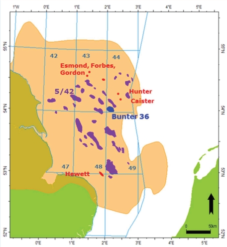
In 2015 the Energy Technology Institute (ETI) selected five potential sites for commercial-scale CO₂ storage in the UK [2]. The Bunter Closure 36 (BC36), located in the Southern North Sea, off-shore the east cost of the UK (Fig 1), was one of the prospects chosen due to its ideal dome structure offering a good storage efficiency, and its strategic location near two important CO₂-generating clusters, the river Thames and the Humber.

The development plan elaborated for the site and the computational model used for the initial assessment are publicly available [3], and have been used to set up the model presented in this study.

Fig. 1. Location of Bunter Closure 36 prospect.

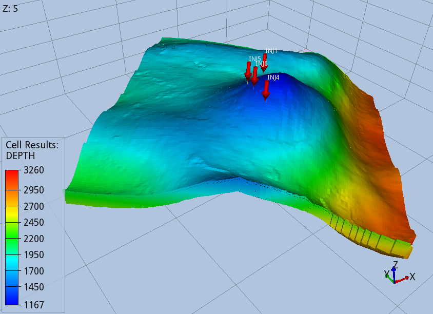
The target layer has a thickness of about 200 m, with the crest of the dome situated at a depth of 1170 m below sea level.

The number and location of the injector wells have been chosen to maximise the injectivity while minimising the pressure build-up to preserve the integrity of the caprock. The maximum pressure permitted has been fixed to 90% of the fracture pressure, which is computed using a fracture pressure gradient value of 0.168 Bar/m.

The four wells selected are all located in the western side of the dome (Fig. 2), a configuration that favours the brine displacement towards the east, and avoids an excessive pressure build-up, which is the limiting factor of the storage capacity of BC36.

Fig. 2. Target layer of Bunter Closure 36 and location of the 4 injector wells.

Each well injects 1.75 Mt (Mega Tonnes) of CO₂ per year, for 56 years, reaching a total capacity of 392 Mt. The well top hole temperature is estimated to be at 4 C, i.e. the sea bed temperature. Well pipe simulations suggest that CO₂ will enter the aquifer at about 12 C [2], where it encounters an average ambient temperature of 45 C.

The Bunter Closure 36 computational model

The computation model, as downloaded from the ETI website, covers an area of 25 x 25 km, and uses a horizontal discretization of 200 x 200 m. Vertically, the computational grid has a variable discretization that goes from 0.5 to 20 m, with refinement in proximity to the impermeable layers, where the CO₂ is expected to accumulate. The total number of active cells is approximately 600,000.

Permeability, porosity and other static data, as well as relative permeability drainage and imbibition curves are those given in the ETI model. The static data required for thermal modelling are not provided, however the properties needed have been estimated with the following values: the rock density is equal to 2350 kg/m³, the rock heat capacity is taken as 1000 J/(kg-K), and thermal conductivity of the saturated rock is given a value of 1.541 W/(K-m).

The surrounding remainder of the aquifer, which has a volume of 270 km³, is connected to the computational model by means of cell volume multipliers applied along the lateral boundaries.

The simulator used for the study is the CO₂ storage option of PFLOTRAN-OGS [4]. This can model a system with two phases (aqueous and vapour) and two components, (CO₂ and water), which can be present in both phases. The partitioning of CO₂ and water in the aqueous and vapour phases is modelled using the correlation of Duan and Sun, [5]. Supercritical CO₂ is characterised using correlations by Span and Wagner [6] and Fenghour et al [7]. The water properties are computed using standard water tables, correcting the density for the presence of dissolved CO₂ and salt [8]. A constant background salt concentration of 4.28 molar is used, which impacts the solubility of CO₂ in brine and brine density. The formulation accounts for molecular diffusion in the aqueous phase, using a diffusion coefficient of 4x10^-9 m²/s, as suggested by Tamimi [9].

Three modelling options are compared to assess the temperature effects:

• Option 1. Isothermal, using an average temperature of 45 C.
• Option 2. A vertical distribution temperature obtained by imposing T = 37.5 C at the crest of the dome (depth of 1167 m) and a thermal gradient of 30 C/km, which remains constant in time.
• Option 3. A full thermal option, where the initial temperature is the same of option 2, but heat conduction and convection are also modelled. Cell volume multipliers are applied to the top and bottom layers so that their heat capacity is increased, and their temperatures remain fixed to the initial values given by the geothermal gradient over the 1000 years simulated. These layers, with nearly-zero permeability, confine the aquifer and model the thermal inertia of the over- and under-burden.

Option 2 accounts for the vertical variation of the temperature in the fluid flow calculations. Option 3 can also model the cooling-down due to the injection.

The computational model simulates the 56-year injection, starting from 2027, and a post-injection phase until 3027, 1000 years from the start of injection.

Results

Three simulations were carried out, one for each temperature modelling option selected. Each run was processed on an Amazon Web Service computational node powered by a 3.0 GHz Intel Xeon Platinum processor with 36 cores. The simulations using options 1 and 2, took approximately 55 minutes, while for the thermal modelling option 3 the computational time was 70 minutes.

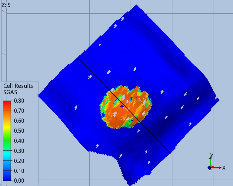
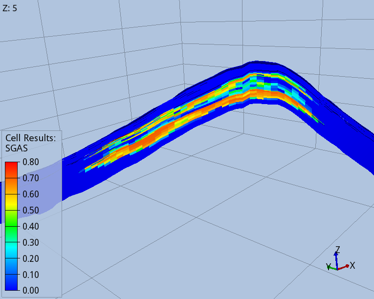
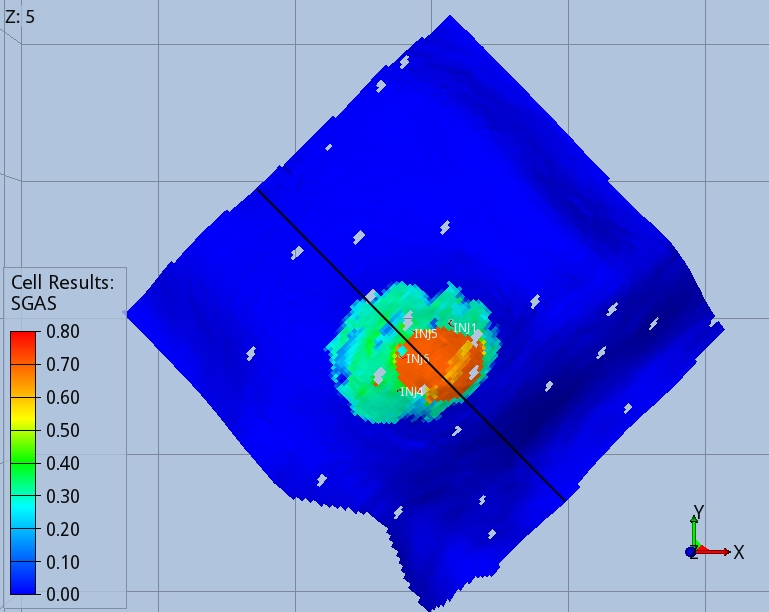
Figures 3 and 4 show the shape of the CO₂ footprint and distribution along a cross section at the end of the injection period, and 1000 years after the injection started. An intra-shale divides the target layer in two sub-layers, which are both completed by the injector wells. The size of the footprint is shown at the top of the deeper sub-layer, as this is affected by a wider CO₂ spread.

Fig. 3.a – CO2 contour in Jan 2083. CO2 footprint with trace of cross section (black line).

Fig. 3.b – CO2 contour in Jan 2083. Gas saturation contour along the cross section marked in figure 3.a.

Fig. 4.a – CO2 contour in Jan 3027. CO2 footprint with trace of cross section (black line).

Fig. 4.b – CO2 contour in Jan 3027. Gas saturation contour along the cross section marked in figure 4.a.

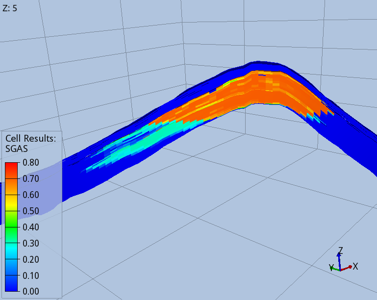The CO₂ migrates upwards until it finds the two impermeable seals present in the target layers. When the injection stops, migration continues towards the crest of the dome, with part of the CO₂ being trapped in the pores of the rock, as shown by the blue trail in Fig. 4. One thousand years after the injection started, 75% of the CO₂ mass is structurally trapped as free gas, 22% is residually trapped, and 5% is dissolved in brine.

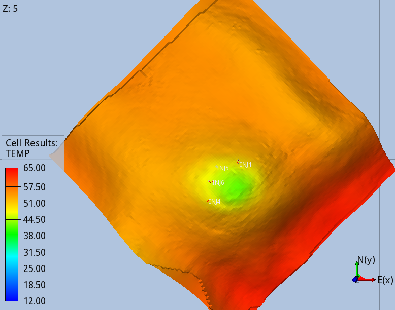
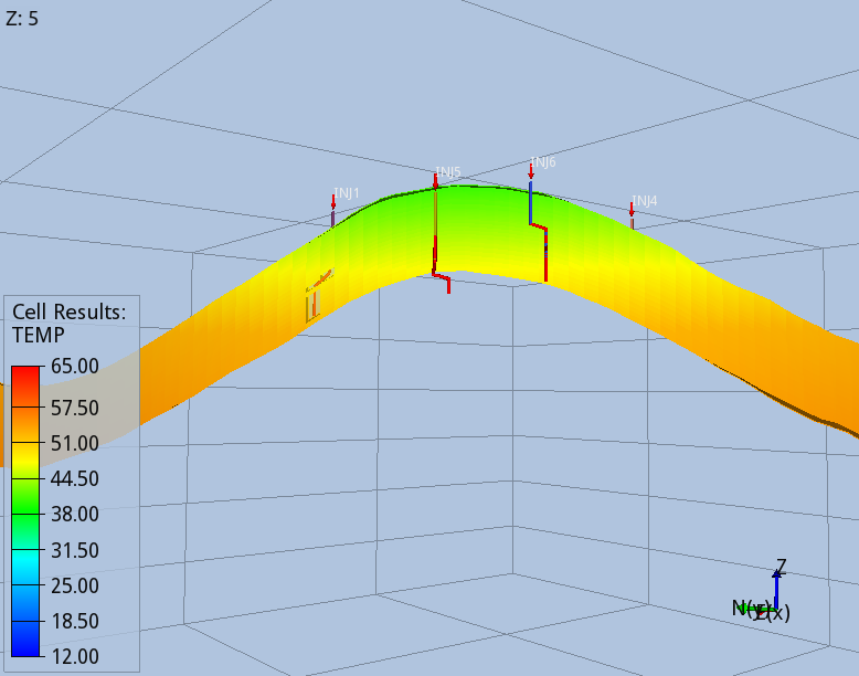
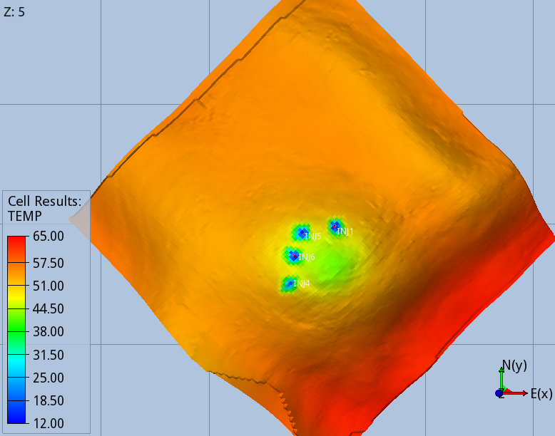
When the full thermal model is run (option 3), the CO₂ entering the aquifer cools down the immediate surroundings of the wells, and the regions swept continuously by the CO₂ stream during the 56 years of injection, Fig 5 and 6.

Fig. 5.a – Temperature contours in Jan 2027, before the injection starts. Top of deeper target sub-layer.

Fig. 5.b – Temperature contours in Jan 2027, before the injection starts. NE cross section between the injector wells.

Fig. 6.a. – Temperature contours in Jan 2083, at the end of the injection. Top of deeper target sub-layer.

Fig. 6.b – Temperature contours in Jan 2083, at the end of the injection. NE cross section between the injector wells.

The modelling options 1, 2 and 3 predict different pore volumes occupied by the CO₂ at the end of the injection. The smallest value is predicted by the full thermal option 3, as the cooler region reached by the temperature front increase the density of the CO₂. While this effect has a minor effect on the CO₂ foot print, it affects significantly the pressure build-up due to the injection, which is the design parameter limiting the storage capacity of the BC36 prospect. Monitoring the pressure below the primary caprock, above one of the injectors, where the risk of fracturing the rock is higher, the thermal run (option 3) predicts an over-pressure ~15% smaller than the one computed by isothermal model (option 1), Fig 7. Very similar values are found for locations above all the other injectors.

Fig. 7 – Pressure vs time in a cell above the injector 1 in the layer just below the primary caprock. Blue, modelling option 1; Red, modelling option 2; Green, modelling option 3.

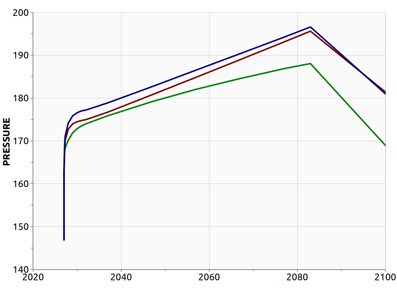When accounting for the time-constant vertical distribution of the temperature, option 2, the pressure initially follows the thermal run (option 3). However, it eventually diverges as the temperature front propagates away from the wells. Once the injection has stopped, the pressure decreases in all cases at slightly different rate, and the region cooled down by the injection gradually recovers the initial temperature due to the heat conduction from the warmer surroundings.

Conclusion

The Bunter Closure 36 prospect is an excellent candidate for large-scale CO₂ storage in the UK, due to its dome structure that provides a four-closure confinement and good storage efficiency. The pressure build-up during injection is a limiting factor for the storage capacity, as this must remain below the fracture pressure to preserve the integrity of the caprock. Since the temperature has a non-negligible effect on the maximum pressure reached during the injection, accurate thermal modelling can help improve the design of the injection strategy.

References

[1] Chadwick, R.A., Arts, R., Bernstone, C., May, F., Thibeau, S., Zweigel, P., 2008. Best Practice for the Storage of CO2 in Saline Aquifers. British Geological Survey, Keyworth, Nottingham (Occasional Publication 14)

[2] Progressing Development of the UK’s Strategic Carbon Dioxide Storage Resource. Constain, ETI, Pale Blue Dot, Axis Well Technology. April 2016.

[3] Strategic UK CCS Storage Appraisal Project, funded by DECC - ETI Open Licence for Materials. D10: WP5A – Bunter Storage Development Plan.

[4] https://opengosim.com/pflotran-ogs-releases.php

[5] Duan, Z. and Sun R. [2003]An improved model calculating CO2 solubility in pure water and aqueous NaCl solutions from 273 to 533 K and from 0 to 2000 bar. Chemical Geology, 193(3–4), 257-271.

[6] Span, R. and Wagner, W. [1996] A New Equation of State for Carbon Dioxide Covering the Fluid Region from the Triple-Point Temperature to 1100 K at Pressures up to 800 MPa,Journal of Physical and Chemical Reference Data, 25(6), 1509–1596.

[7] Fenghour, A,Wakeham, W.A.,andVesovic, V. [1998] The Viscosity of Carbon Dioxide. Journal of Physical and Chemical Reference Data, 27, 31-44.

[8] Duan, Z., Hu, J., Li, D., and Mao, S. [2008] Densities of the CO2-H2O and CO2-H2O-NaCl Systems up to 647 K and 100 MPa, Energy & Fuels, 22, 1666–1674.

[9] Tamimi, A., Rinker, E. B., and Sandall, O.C. [1994] Diffusion Coefficient for Hydrogen Sulfide, Carbon Dioxide, and Nitrous Oxide in Water over the Temperature Range 293-368 K.Journal of Physical and Chemical Reference Data, 39(2), 330-332.