Is temperature an important parameter to consider in CO₂ injection?

As anthropogenic CO₂ emission must be cut to mitigate global warming, the carbon capture utilization and storage (CCUS) will play an important role to decarbonise energy generation from fossil fuel in the transition period to renewable energy, and to cut emissions of heavy industries for which zero-carbon alternatives do not exist yet, e.g. cement, etc.

CO₂ has already been used for years in the US to recover oil, due its very good miscibility with hydrocarbons, in what it is called CO₂ enhanced oil recovery (CO₂-EOR). However, up to now, this technology has been limited due to the high costs and to the limited availability of CO₂. For the same reason, CO₂-EOR operations always tried to maximise oil production with the minimum amount of CO₂ injected. In a scenario in which CO₂ is abundant, and CO₂-EOR is used in combination with CO₂ storage, the problem can change to maximising the amount of CO₂ stored, while improving the oil recovery. This study assesses the CO₂ injection temperature as one of the parameters that can change the patterns followed by CO₂ when used in EOR, and demonstrates its sensitivity with numerical simulations. The idea has already been presented using thermal compositional simulators [1]. However, the application of this type of simulators to three-dimensional full scale reservoir problems is not realistic due to the high computational cost. In this study a simpler approach based on a Thermal Todd-Longstaff model is presented, demonstrating its ability to describe temperature sensitivity.

Problem Setup

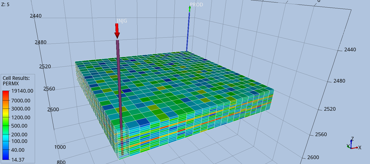
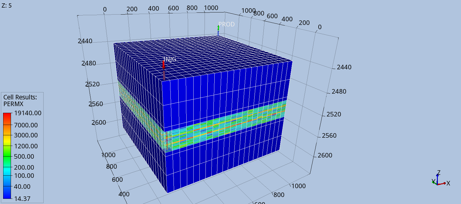
As proof of concept, a small problem has been defined with 20 x 20 x 15 cells, and a space discretisation of DX = DY = 50 m and DZ = 2 m, therefore the domain size is 1000 m x 1000 m x 30 m. The top of the target layer is at a depth of 2500 m.

The porosity and permeability are made up, however they resemble the geology of a cross section of a real Norwegian reservoir considered for CO2-EOR [1].

The porosity is constant and equal to 0.3. The permeabilities were obtained using base values of PERMX = PERMX = 200 mD and PERMZ = 25 mD. Two high permeability channels were introduced, applying permeability multipliers of 10 and 15 in layers 5 and 10. The final distribution is obtained applying a Dykstra-Parsons coefficient of 0.5, which makes the permeability field heterogeneous for a more realistic representation.

Initially the domain is saturated with light live oil, with a connate water saturation of 0.2. The relative permeabilities and the oil and gas properties are taken from the SPE5 case [2], given for a temperature of 70 C. A temperature dependency is introduced for the oil viscosity, by providing saturated oil viscosities at 2 C, about four times larger with respect to the viscosity values given at 70 C.

The solvent is pure CO₂ with pressure and temperature dependent properties computed using the Span and Wagner EOS [3], while viscosity uses a model from Fenghour et al. [4]. Initial pressure is 275 bars with a small variation due to hydrostatic equilibration. Initial temperature is set to 70 C.

Injector location and condition

A fully completed injector is located at the column (1,1), injecting 230,000 tons per year of CO₂. The injection starts two year after depletion, and is carried out for 28 years. The total simulated time is 30 years.

The CO₂ delivery pressure and temperature can vary significantly depending on many factors, including economics, distance to cover, surrounding conditions, etc. Peletiri et al [5] provides a literature review of existing pipeline, indicating ranges of [85-150] bars and [15-44] °C, for the operating pressure and temperature. A minimum pipeline pressure of 85 bars is supported to ensure that CO₂ remains in a dense phase, while CO₂ is often warmed up or cooled down to optimise transport conditions. For this study, a surface pressure of 85 bars and two temperature scenarios were considered, 5 C (cold injection) and 70 C (warm injection). These values are used to compute the energy of the CO₂ from the delivery pipeline or from the outlet of a compressor.

Achieving the required bottom hole pressure would require very little or no compression from the surface, as the hydrostatic pressure helps significantly to push the fluid into the reservoir, especially in the case of lower injection temperature for which the CO₂ has a liquid-like density. The target surface temperature can be achieved warming up or cooling down the fluid, depending on delivering conditions.

In the well tubing from the surface to the target layer, friction losses and heat conductions with the surrounding environment were ignored. Potential energy changes were also neglected, accounting only for compression effects on the fluid energy changes.

Once the mass of CO₂ to inject has been fixed, the first and most important effect of varying the temperature is to vary the reservoir volume injected. In fact, CO₂ density decreases as the temperature increases. For an approximate estimate of the reservoir volumetric injection rates in the two injection temperature scenarios, the average bottom hole pressure (BHP) and temperature (BHT) were taken from the simulation results. An average BHP of ~ 86 bars can be applied to both cases, while two different average BHTs are observed:

Tinj ( °C)	BHP average (Bar)	BHT average (° C)	CO2 density (kg/m3)	Qres (m3/day)
70	86	70	194	3240
10	86	10	909	692

Producer location and condition

A producer was placed in the opposite corner of the injector (column 50x50), with an oil target surface rate of 1907 m³/day, and a minimum bottom hole pressure limit (BHPL) of 80 bars. The producer is completed in 8 layers in the lower part of the reservoir, and it is open from start, when depletion begins. Note that a BHPL of 80 bars was chosen to ensure that CO₂ remains in its dense phase also at reservoir conditions.

Thermal Boundary Conditions

To include the effect of the boundary heat conductions, three layers were added above and below the target layer, with variable vertical spacing (DZ = 6, 30, 30 m). These layers were assigned a very small porosity of 0.001 and zero permeabilities in all directions, as they are considered impermeable.

After some preliminary simulation to understand the temperature propagation into the heat condition boundaries, the most external layers (last of three in each side) were assigned a very high heat capacity to freeze their temperature to the initial value (i.e. 70 C).

Results and comments

When the simulation starts, only the producer is open, and the depletion causes a rapid decline of the pressure that crosses the bubble point. Reservoir gas comes out of solution forming a cap in the the top layers, Fig 1.

Fig. 1 – Reservoir gas saturation at 2 years before solvent injection starts

The CO₂ injection start two years after depletion began, and the CO₂ tends to channel in the upper high permeability layer, with tendency to fingering everywhere due to the high mobility ratio with respect to the oil. Different CO₂ patterns are observed in the two cases for injection temperatures of 5C and 70 C. Figures 2 to 7 below show solvent saturation and temperature contour plots for the two cases at three different times: (i) 2 years and 6 months, (ii) 12 years and (iii) 30 years.

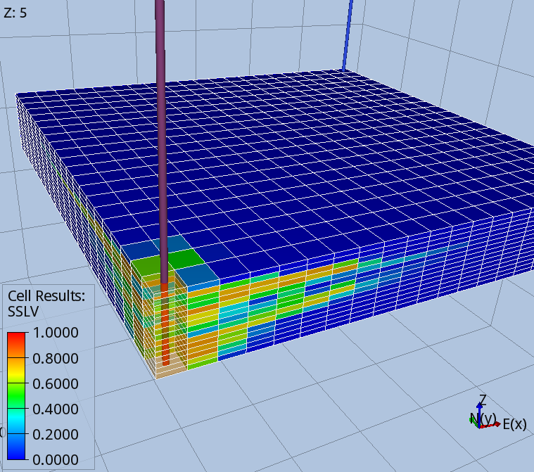
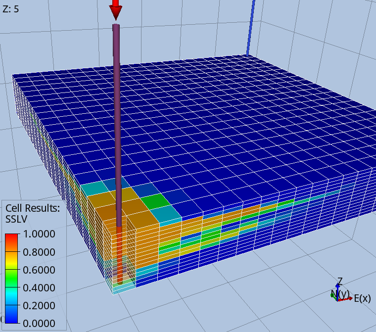   Fig. 2 – Solvent saturation at 2 years and 6 months: left 5C injection, right 70C injection

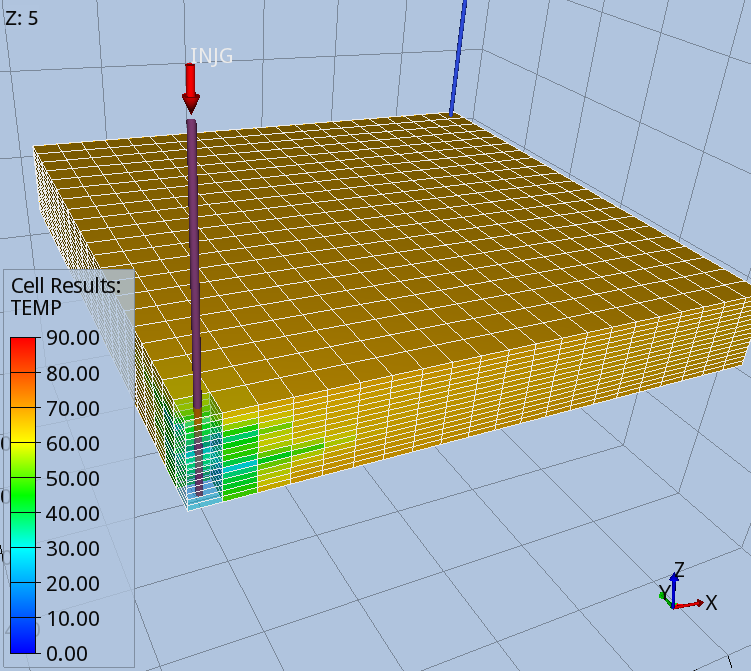
  Fig. 3 – Solvent saturation at 2 years and 6 months: left 5C injection, right 70C injection

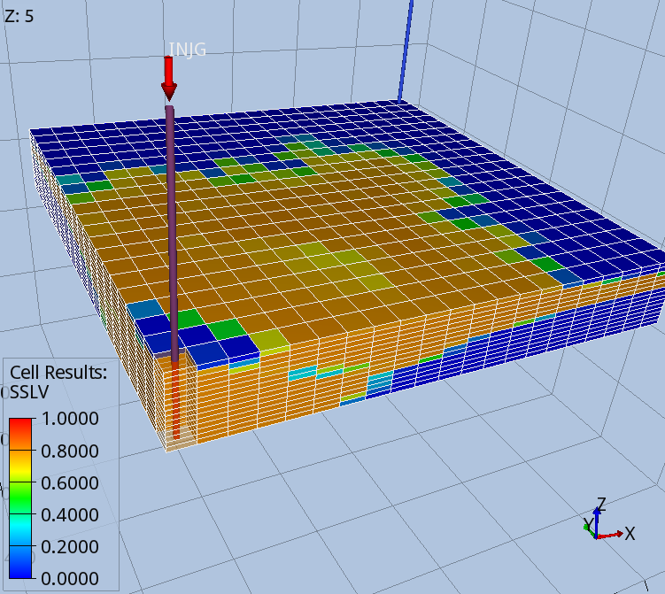
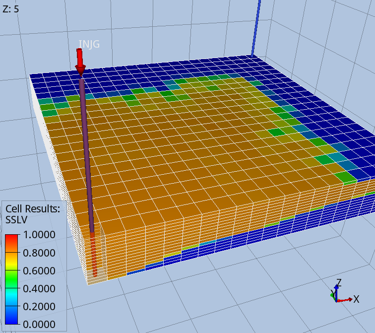  Fig. 4 – Solvent at 12 years: left 5C injection, right 70C injection

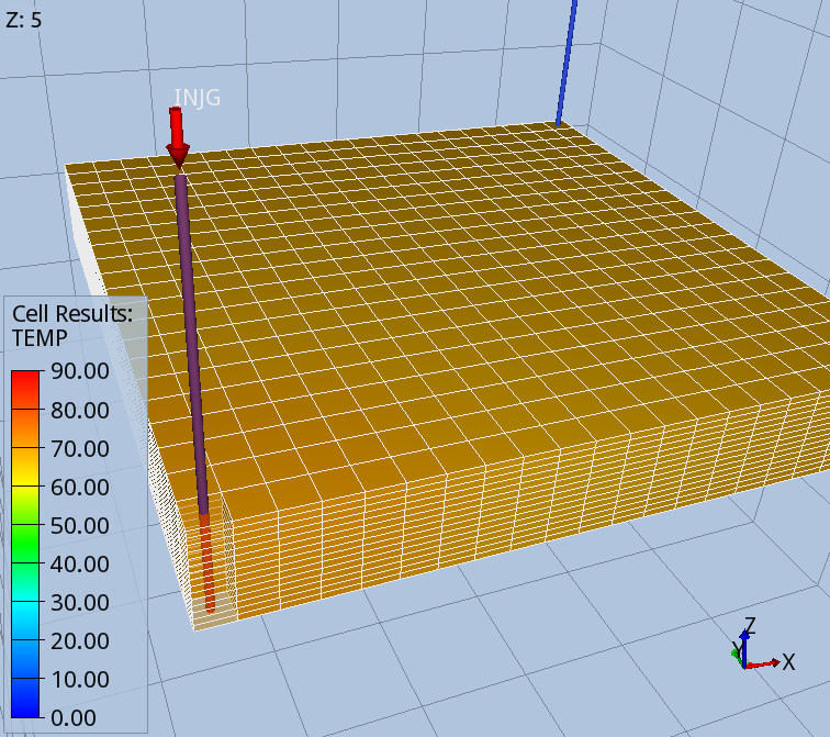  Fig. 5 – Temperature at 12 years: left 5C injection, right 70C injection

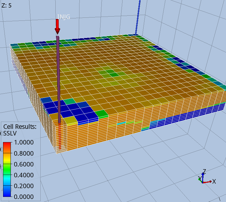
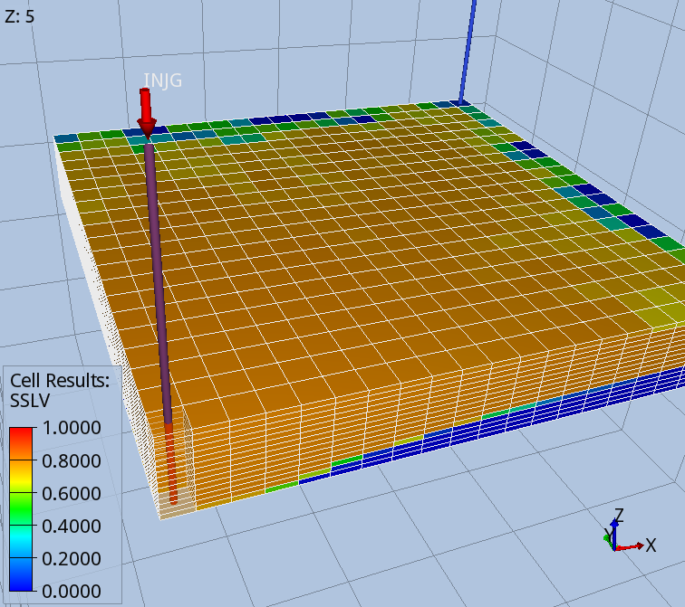  Fig. 6 – Solvent at 30 years: left 5C injection, right 70C injection

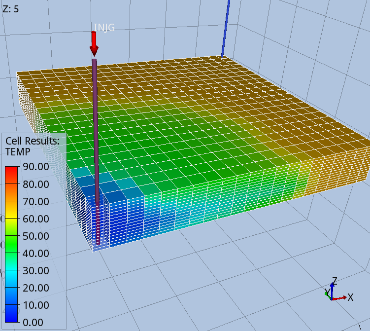
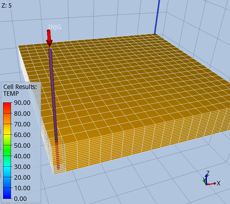  Fig. 7 – Temperature at 30 years: left 5C injection, right 70C injection

In the cold injection the CO₂ tends to by-pass more cells in the upper part of the domain, due to the tendency to sink, as at lower temperature the CO₂ density gets larger than the density of the light oil used in this case. However, it also has the tendency to sweep lower layers, which instead are skipped by the warm injection, as lighter CO₂ tends to migrate more quickly to the top.

Colder CO₂, at the prevailing pressure of this study (~86 bars for both cases), results in an important increase of both density and viscosity from 70 C to 5 C.

Tinj ( °C)	Pressure (Bar)	CO2 density (kg/m3)	CO2 viscosity (cP)
70	86	194	0.02
5	86	938	0.10

With the oil density ranging between [370 – 765] kg/m³ in this problem, the higher density of the CO₂ at 5 C explains why the solvent reaches more lower layers in the cold injection scenario. On the other hand, the lower viscosity at 5 C reduces the mobility and therefore the migration of the solvent towards upper layers (and in theory fingering, not well captured with the resolution of this model).

In the solvent saturation at 30 years for the cold injection case, the upper layers close to the injector show a region at low solvent saturation, which contains both oil and reservoir gas. Some of this oil was initially by-passed by the solvent flood, but other migrated from underneath layers as lighter than cold CO₂. Reservoir gas comes out of solution of this trapped oil as the pressure keeps falling. Some details on these near-well effects are reported in appendix.

The oil residual saturation at 30 years for the two cases are shown in figure 8 below:

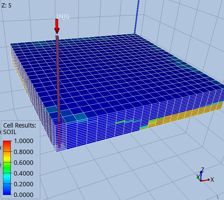
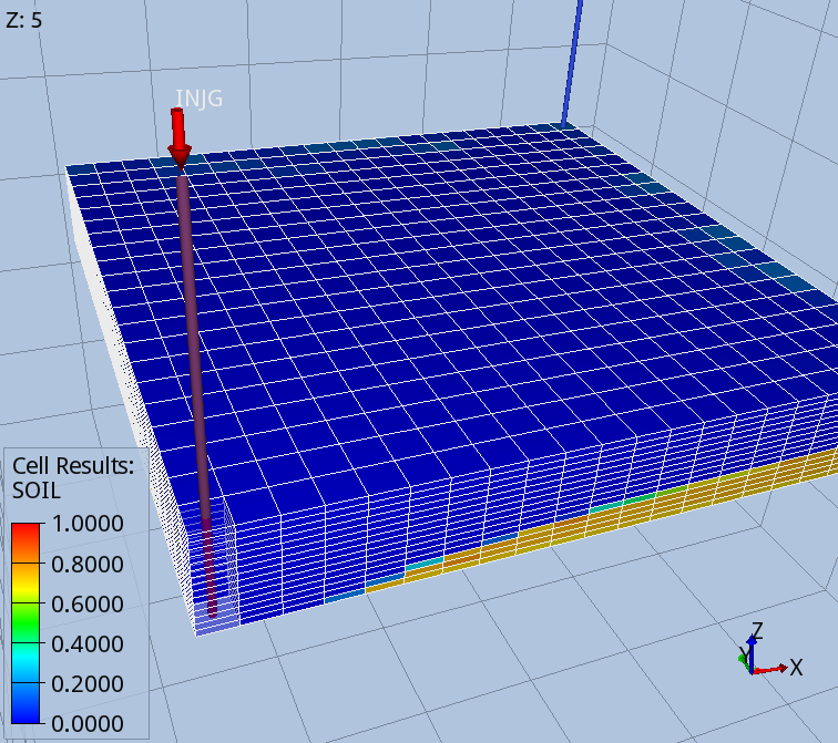  Fig. 8 – Oil saturation at 30 years: left 5C injection, right 70C injection

The effect of the temperature in the aquifer above and below the target layer are shown in figure 9.

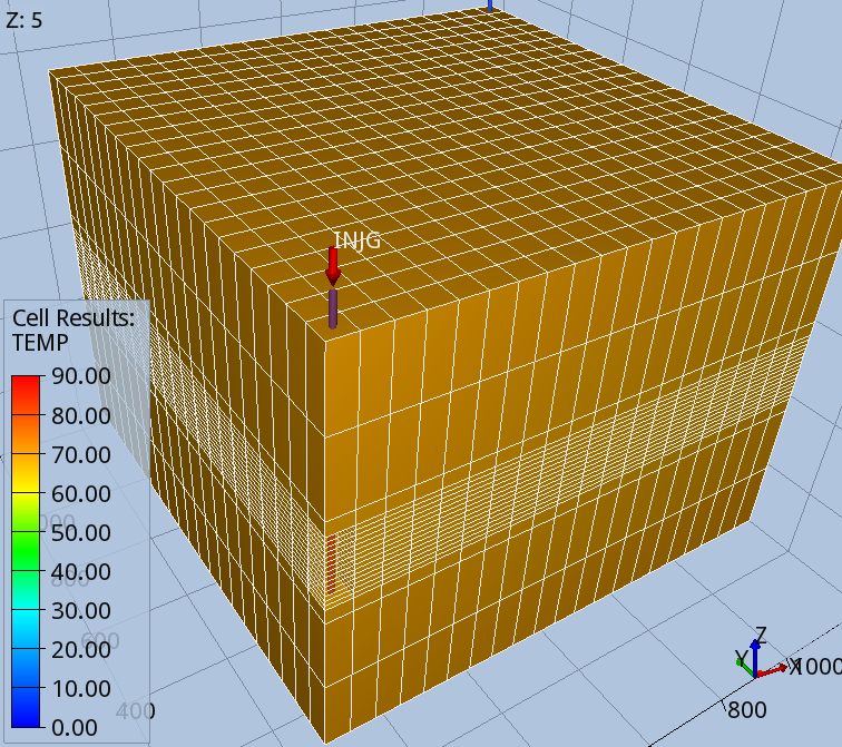  Fig. 9 – Temperature at 30 years: left 5C injection, right 70C injection

The warm injection occurs mainly at reservoir initial temperature, and has no important effects. However, the cold injection, at a considerably lower temperature than the one initially found in the reservoir, cools down significantly the aquifers above and below the target layers, especially in the region close to the well.

The oil and solvent total production, the solvent production rate, and the Solvent-Oil ratio are shown below.

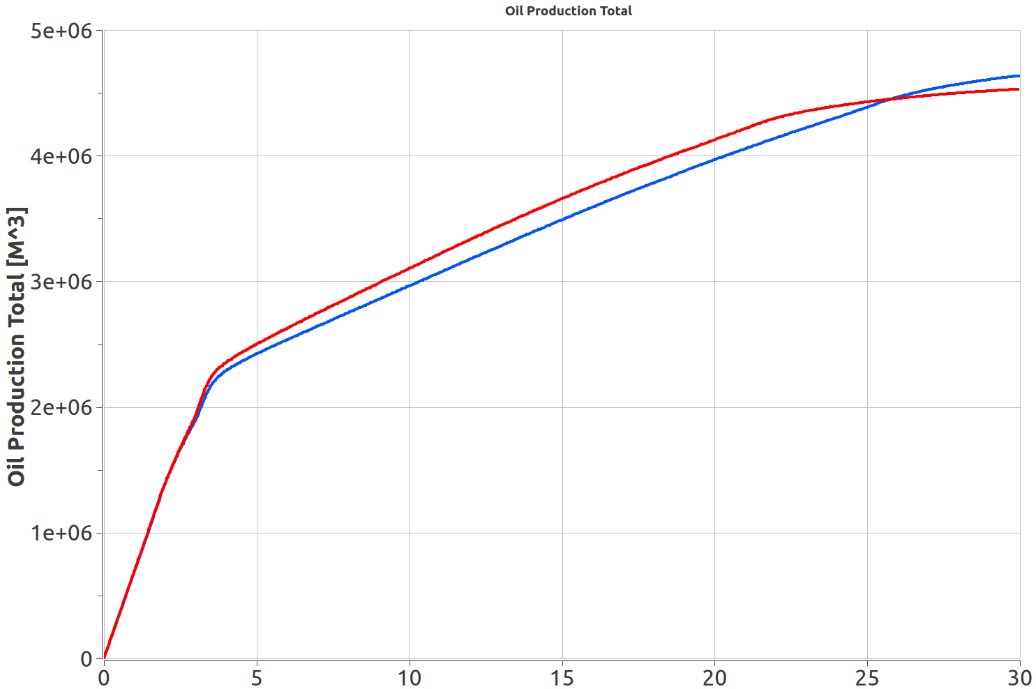
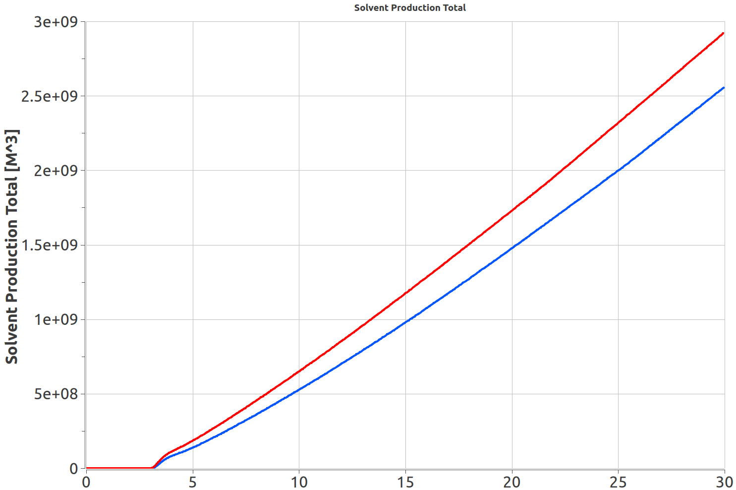  Fig. 10 – Oil (left) and Solvent (right) Production Totals: blue 5C injection, red 70C injection.

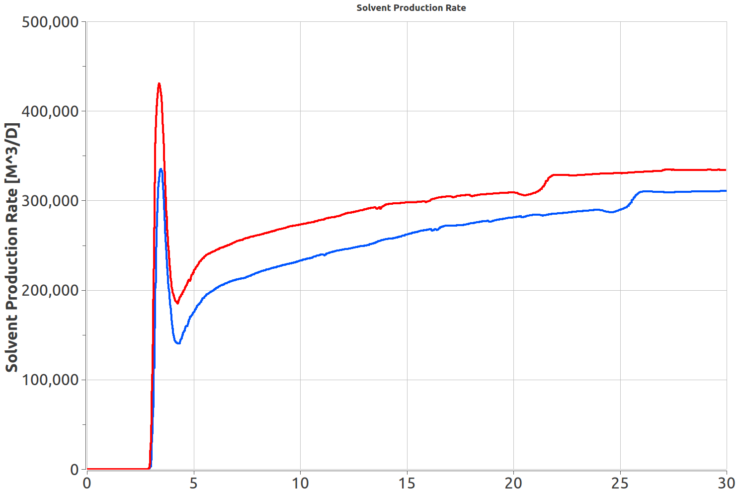
  Fig. 11 – Solvent Production Rate (left), Solvent-Oil ratio (right). Blue 5C injection, red 70C injection.

Solvent breakthrough is observed at year 3, one year after injection started in both cases. The oil production in the warm injection case is overcome by the cold injection scenario only in the last 5 years. The warm injection produces more CO₂ back during the entire 30-year period.

Conclusion

As more solvent reservoir volume is injected by the warm injection, a better total oil production is achieved in the short and medium periods. However, would one consider a prolonged CO₂ injection, as it could be for the case of storing CO₂ while recovering oil, a better sweeping can be achieved and ultimately a better total oil recovery by cold injections, in agreement with [1]. The lower temperature injection also produced a lower amount of solvent back, explained by a smaller reservoir volume injected and better exploitation of the deeper layers. Temperature seems to be one of the designing parameters to consider when planning for both CO₂ storage and CO₂-EOR. It must be said that a stress analysis would be required to understand if thermal shock could endanger the integrity of the reservoir.

References

[1] B. Nazarian et al. (2014) , Composition Swing Injection for CO₂ Storage and EOR, SPE-171798-MS.

[2 ] Killough, J. E., & Kossack, C. A. (1987). Fifth Comparative Solution Project: Evaluation of Miscible Flood Simulators. Society of Petroleum Engineers. doi:10.2118/16000-MS

[3] Span, R., Wagner, W. (1996), A New Equation of State for Carbon Dioxide Covering the Fluid Region from the Triple-Point Temperature to 1100 K at Pressures up to 800 MPa, J. Phys. Chem. Ref. Data, 1996, 25, 6, 1509–1596.

[4] Fenghour, A & Wakeham, William & Vesovic, V. (1998). The Viscosity of Carbon Dioxide. Journal of Physical and Chemical Reference Data - J PHYS CHEM REF DATA. 27. 31-44. 10.1063/1.556013.

[5] Suoton P. Peletiri et al. (2018), ‘CO₂ Pipeline Design: A Review’, Energies 2018, 11, 2184.

 

Appendix - Near well effects

To explain the changes in solvent saturation in the top layers close to the injector, it is worth taking a close look at what happens in cell (2,1,1).

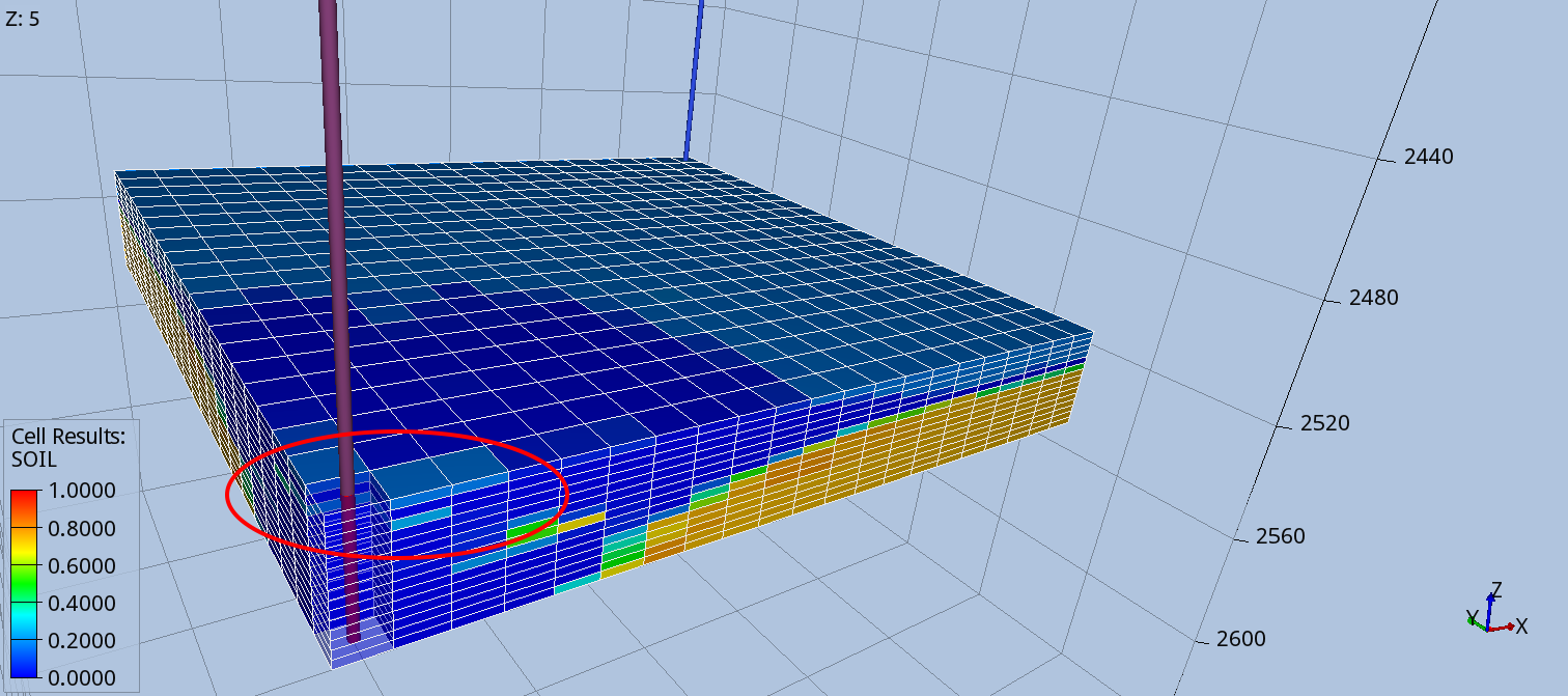
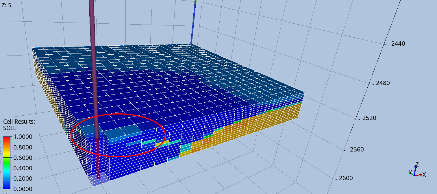  Fig. A1 - Oil saturation at t = 5 years (left) and t = 8 years (right), for the cold injection case.

Column (2,1) shows some oil initially by-passed by the solvent flood. Here, there is some oil moving upwards as CO₂ sinks. This can be better observed by looking at the saturation history of one of the top cell near the well (2,1,1)

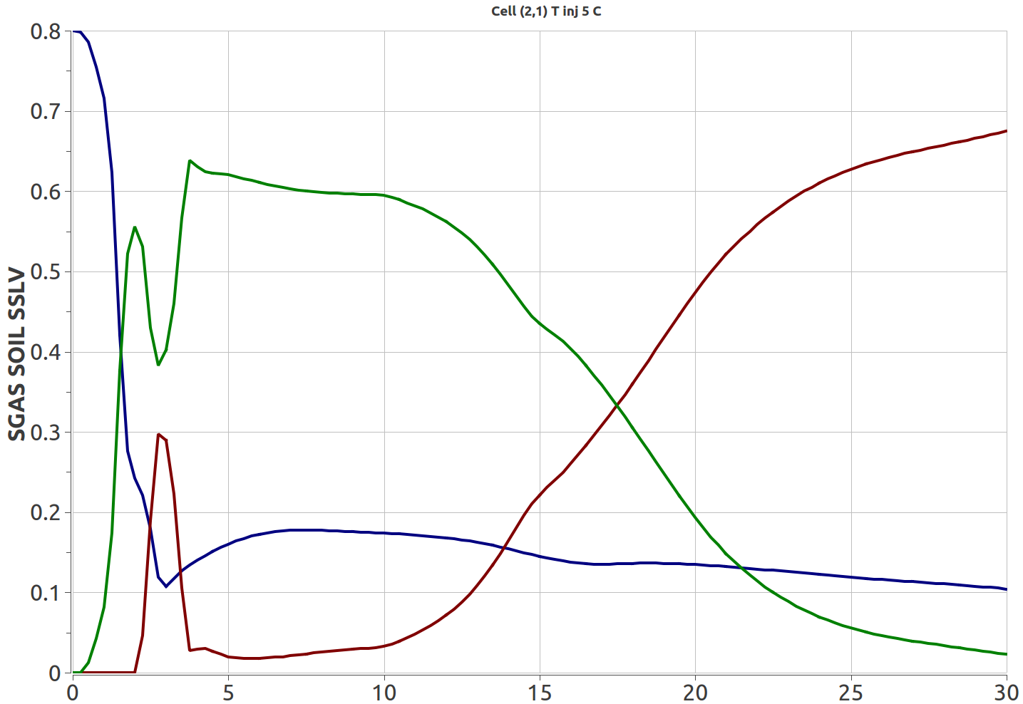Fig. A2 – Saturation history for cell (2,1,1), Tinj = 5 C. Blue = oil; Red = solvent; Green = gas. Swc ~ 0.2

Different phases can be distinguished in the plot above:

• 0-2 years: Gas coming out solution due to depletion

• from 2 years (injection start) to 2.75 years (first solvent saturation peak, Ss ~ 0.3): Solvent injection displays both oil and reservoir gas at a faster rate than gas coming out of solution

• from 2.75 to 3.75 years (fast Ss decline): Most solvent injected goes into the preferential high perm layer underneath the top layers. The top layer close to the well, and so the cell (1,2,1) receives little CO₂ flooding, and as the pressure decline due to depletion is still strong, the gas coming out of solution is displacing the solvent.

• from 3.75 years to about 7.5 years: The pressure decline due to depletion flattens, and oil is being displaced by the solvent at low rate. In this phase Ss sees a small decline while the Oil saturation is growing gently. This is due to oil in the underneath layers which, initially by-passed by CO₂ flooding, is now moving upwards, as lighter than the solvent due to the low temperature close to the well.

• From 7.5 year onwards: pressure is nealry constant, no more oil rising from underneath layers, a slow and continuous oil and gas displacement by the solvent is the main phenomena until the end.